Pulse Propagation Modeling in Dispersion Managed Optical Fibers

The following is an excerpt from a group project completed in my finial year at the University of Aberdeen. Dr. Kaliyaperumal Nakkeeran supervised the project. The group project title was Simulation of Pulse Propagation in Optical Fiber Transmission Systems. The aim of the project was to simulate the pulse propagation in dispersion managed (DM) optical fiber transmission systems. Effects like optical losses, group-velocity dispersion and self-phase modulation are analyzed in this project. Part of my contribution to the project was the production of a MATLAB simulation of the pulses’ propagation through the wave-guide.

Introduction

The aim of this group project was to simulate the pulse propagation in dispersion managed (DM) optical fibre transmission systems. Effects like optical losses, group-velocity dispersion and self-phase modulation are analyzed in this project.

Nonlinear pulse propagation in a fiber can be described by the generalized nonlinear Schrödinger equation (NLSE), which has the form,

Wwhere ψ(z, t) is the slowly varying envelope amplitude of the electric field measured in units of square root of Watts at position z, at time t. Subscript z or t denotes the partial derivative with respect to that letter. β₂(z) and β₃(z) represent the second and third order dispersion coefficients respectively. γ(z) represents the strength of the nonlinearities.

Split Step Fourier Method

Description

The non-linear Schrödinger equation describes the propagation of the wave through an optical wave-guide. The equation is described in Equation 2‑1. The equation represents the non-linear response of the dielectric to the electric field of the propagating light wave.

The non-linear Schrödinger equation consists of two main components, the linear component as described in Equation 2‑2 and the non-linear component as described in Equation 2‑3. The non-linear and the linear components of the equation is solvable separately however non-linear Schrödinger equation does not have a simple solution.

If the only a step h is taken along the waveguide z, then the linear and non-linear components can be treated separately resulting in only a small numerical error.  These steps are illustrated in Figure 2‑1. 

In each step in the splits-step method there are three operations, involving the non-linear and linear components. The non-linear transfer function is applied from to , then from to . The linear transfer function is then applied from to . This is illustrated in Figure 2‑2.

Derivation

Linear Component

The linear component of the operation can be obtained from the non-linear Schrödinger’s equation (Equation 2‑4).

The second derivative of the amplitude can be substituted with the Fourier transform as described in Equation 2‑5,

Rearranging for  gives Equation 2‑6,

Integrating  with respect to  between  and , and with respect to  over o to h as in Equation 2‑8,

giving Equation 2‑9.

Re-arranging into a transfer function between the current step and the next step values as in Equation 2‑11,

When implemented in MATLAB Equation 2‑11 takes the form:

i = sqrt(-1);

A = A.*exp(-alpha*(h/2)+i*beta/2*w.^2*(h/2));

Non-Linear Component

The non-linear component of the operation can be obtained from the non-linear Schrödinger’s equation (Equation 2‑12).

The equation is then rearranged in terms of , as in Equation 2‑13

Integrating  with respect to  between  and , and with respect to  over 0 to h as in Equation 2‑14,

giving Equation 2‑15

Re arranging into a transfer function between the current step and the next step values as in Equation 2‑18,

When implemented in MATLAB Equation 2‑18 takes the form:

i = sqrt(-1);

A = A.*exp(i*gamma*(abs(A).^2)*h);

Demonstration of Algorithm

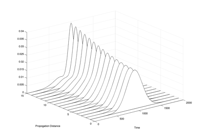
The MATLAB program is demonstrated in Figure 2‑2. In this graph a generic pulse is shown evolving as it propagates through a glass wave-guide.

Flow Diagram of Procedure