As part of my undergraduate degree at the University of Aberdeen, I completed an undergraduate thesis. In my thesis, I considered the concept of a multi-static passive radar system capable of tracking commercial civil aircraft using transmitters of opportunity.
One possible obstacle for a multi-static TDOA radar system is solving a system containing multiple targets. Solving the system quickly enough to enable a quick refresh rate, and real time operation is envisioned as a major obstacle as it could be prohibitive in terms of cost. In this entry I will discuss system complexity while tracking multiple targets, discuss the difference between real and ghost targets and approaches to reduce overall system complexity.
System Complexity
Given the real-time requirements of the system and that computing resources available to any system are finite, it is important to have an idea of how expensive in terms of computing power the system might be. The system will be required to compute the location of all the targets in range and again for each refresh to maintain a real-time view of the targets of interest. Using an indiscriminating brute force approach would be inefficient in terms of computing power. Solving the system in this way has a complexity of approximately
![]() ,
,
for a 2D system. A 3D system has the approximate complexity of
![]() .
.
Where ![]() is the number of targets and
is the number of targets and ![]() is the number of unique transmitter-receiver pairs in the system. Using an alternative approach the approximate complexity of the system could be reduced to
is the number of unique transmitter-receiver pairs in the system. Using an alternative approach the approximate complexity of the system could be reduced to
![]() .
.
Target Solutions for Multiple Targets
Locating multiple targets is difficult, as multiple returns will be detected from each transmitter. For a system using a 2D position algorithm and 3 transmitters as described in previously, the number of possible target solutions can be shown using Equitation 4.

Where n is the number of returns, excluding the direct path signal from each transmitter. For a system using a 3D positing algorithm using 4 transmitters as described previously, the number of possible target solutions can be shown using Equitation 5.

Where n is the number of returns, excluding the direct path signal from each transmitter. In this thesis, two possible methods are presented to reduce the number of possible target solutions. The first method is to analyze the behaviour of the possible solutions. The second is the use of additional transmitters to test the possible targets.
Tracking of Multiple Targets in 2D
To analyze system performance when tracking multiple targets, a simulation was devised tracking two simulated targets. The parameterized targets vectors are shown in Equation 6 for target 1 and Equation 7 for target 2. The target vectors are chosen to demonstrate the tracking two aircraft with different bearings and velocities.


The simulation runs from ![]() to
to![]() .
.
There are two returns from each transmitter not including the direct path signal, as there are two targets as shown in Table 1.
| Transmitter | Returns |
|---|---|
| 1 | T1_1, T1_2 |
| 2 | T2_1, T2_2 |
| 3 | T3_1, T3_2 |
Initially the system does not know which return corresponds with which target so every combination is plotted. As per Equation 4, there are 8 possible solutions for a system tracking 2 targets using 3 transmitters. The 8 possible solutions are listed in Table 2.
| Trace | Positing Arguments | Label |
|---|---|---|
| 1 | T1_1, T2_1, T3_1 | Target 1 |
| 2 | T1_1, T2_1, T3_2 | Ghost 1 |
| 3 | T1_1, T2_2, T3_1 | Ghost 2 |
| 4 | T1_1, T2_2, T3_2 | Ghost 3 |
| 5 | T1_2, T2_1, T3_1 | Ghost 4 |
| 6 | T1_2, T2_1, T3_2 | Ghost 5 |
| 7 | T1_2, T2_2, T3_1 | Ghost 6 |
| 8 | T1_2, T2_2, T3_2 | Target 2 |
The traces are plotted in Figure 1. The traces representing genuine targets are coloured blue Target 1 and green Target 2. In Figure 1 the traces that consist of components of target 1 and target 2 are shown to have wild trajectories. These are clearly out with the performance of any aircraft. This is further analyzed in Figure 2.
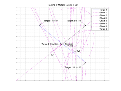
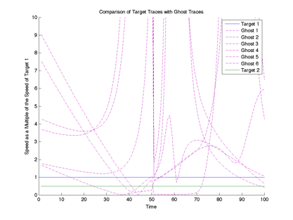
The magnitude of the possible targets as a multiple of the constant speed of target 1 are plotted in Figure 2. The Ghost traces can be clearly distinguished from the genuine targets as their speed is magnitudes higher that that of the fastest genuine target.
Analyzing Possible Target Behavior
This solution exploits the limited range of behaviour that genuine targets show. A false target can be identified when they show behaviour that is not within the range expected from a genuine target. Components such as velocity, position, acceleration and change in direction can be used to distinguish targets.
Analyzing Possible Targets with Additional Transmitter References
Additional transmitters can be used to corroborate possible target solutions. Using a 2D positioning algorithm to track two targets, the result is eight possible solutions as described in Equation 4. For each of these possible targets, the theoretical bi-static range is calculated for the receiver and additional transmitter giving the TDOA for each target. The synthesized TDOA is then compared to the actual returns from the additional transmitter. The error is defined as the difference between the TDOA of the synthesized return and the actual returns from the additional transmitter. As there are two targets, there are two returns received from the additional transmitter. This means that each synthesized TDOA has to be compared with two returns from the additional transmitter. Genuine targets will be distinguished from false targets, as they will have a zero difference from their corresponding return from the additional transmitter.
Corroboration with a Fourth Transmitter
An additional transmitter can be used to corroborate the possible solutions. All the possible solutions for returns describe in Table 3 are calculated as in Table 4.
| Transmitter | Returns |
|---|---|
| 1 | T1_1, T1_2 |
| 2 | T2_1, T2_2 |
| 3 | T3_1, T3_2 |
| 4 | T4_1, T4_2 |
| Target Solution | Positing Arguments | Label |
|---|---|---|
| $1 | T1_1, T2_1, T3_1 | Target 1 |
| $2 | T1_1, T2_1, T3_2 | Ghost 1 |
| $3 | T1_1, T2_2, T3_1 | Ghost 2 |
| $4 | T1_1, T2_2, T3_2 | Ghost 3 |
| $5 | T1_2, T2_1, T3_1 | Ghost 4 |
| $6 | T1_2, T2_1, T3_2 | Ghost 5 |
| $7 | T1_2, T2_2, T3_1 | Ghost 6 |
| $8 | T1_2, T2_2, T3_2 | Target 2 |
| Target Solution | T4_1 | T4_1 | Label |
|---|---|---|---|
| $1 | Target 1 | ||
| $2 | |||
| $3 | |||
| $4 | |||
| $5 | |||
| $6 | |||
| $7 | |||
| $8 | Target 2 |
Using the known locations of the additional transmitter and receiver, the bi-static ranges are calculated for each possible target solution. Using the bi-static ranges, the equivalent TDOA timings are calculated. These are then compared to the actual returns received from the additional transmitter T4_1 and T4_2 as shown in Table 5. All solutions that have an equivalent TDOA that is not close to equal to the measured bi-static ranges T4_1 and T4_2 can be excluded. The remaining two are the genuine target solutions.
1 reply on “Multiple Object Tracking in a Multi-Static Radar System”
hi,
I am working with TDOA measurements and I would like to tkae a llok in you scripts,
BR
Marcelo